What this article covers
- The interface sets the floor. Thermal noise across the electrode-skin contact moves by a factor of five between day 1 and day 14, and no amplifier choice recovers it.
- Guard traces are about potential, not resistance. Board surface leakage at 30 nA against a dried electrode becomes 9 mV of wandering offset.
- Noise reaches the classifier as distribution shift. Motion artefact resembles ventricular tachycardia, and the model fails with high confidence rather than low.
A cardiologist reading a 21-day study never sees your noise floor. She sees a strip, a label under it, and a number at the top of the report telling her what fraction of the recording the system could analyse. That number is where your front end shows up, and it is the only place it shows up.
We keep coming back to this because the failure is silent. A noisy acquisition chain produces a report that looks finished, with a percentage the reader has no reason to interrogate, and the hours it quietly discarded are not distributed evenly across the recording.

The signal you are trying to hold
On a single-lead chest placement, the QRS complex arrives somewhere between 0.5 and 2 mV depending on the vector you picked and the patient in front of you. The P wave arrives at 50 to 150 µV. In an older patient with atrial disease it can sit lower.
Atrial fibrillation classification rests on two observations: organised P waves have disappeared, and the RR intervals have gone irregular. You can pull RR intervals out of a mediocre trace, because R peaks are large and the detector only needs their timing. P waves give you nothing to work with once the floor comes up.
That ratio, and not a headline accuracy figure quoted from someone else's recordings, is what your model inherits.
Start with the part you do not control
Before any component you selected, the patient's skin sets a floor. Thermal noise across the electrode-skin interface follows the Johnson-Nyquist relation,1 and you can compute it in one line.
| Electrode-skin impedance | Noise (rms) | Noise (p-p) |
|---|---|---|
| 10 kΩ · prepped, fresh gel | 0.16 µV | 1.1 µV |
| 20 kΩ | 0.23 µV | 1.5 µV |
| 100 kΩ | 0.51 µV | 3.3 µV |
| 300 kΩ · dried hydrogel, day 14 | 0.88 µV | 5.8 µV |
Swipe the table sideways to see all columns.
The interface alone moves your floor by a factor of five across a three-week wear period, and no amplifier selection recovers it. Skin preparation and hydrogel chemistry buy you more headroom than a better front-end IC does. We spent longer on electrode selection than on the amplifier for exactly this reason.
Impedance also decides which amplifier specification matters. Voltage noise dominates at low source impedance. Current noise multiplied by source impedance dominates at high source impedance, so a part with excellent voltage noise and mediocre current noise degrades through the wear period while a datasheet comparison at 10 kΩ tells you nothing about it.
The noise you build in yourself
Surface leakage across the board arrives first. Take a 3 V rail sitting 2 mm from an input node with 100 MΩ of surface resistance between them, which is what a fingerprint and a week of humidity in Gorakhpur will give you. That path injects 30 nA. Against a 300 kΩ electrode, 30 nA becomes 9 mV of wandering offset, three orders of magnitude above the P wave you were trying to resolve.
A guard trace fixes this by removing the potential difference rather than the leakage path. Drive a ring at the input common-mode voltage, surround both input nodes with it, and the leakage current has nowhere to go because nothing across that gap has a voltage across it. The rule we hold to on every layout: no net at a different potential touches an input node's guard boundary, on any layer, including the layer nobody looks at.
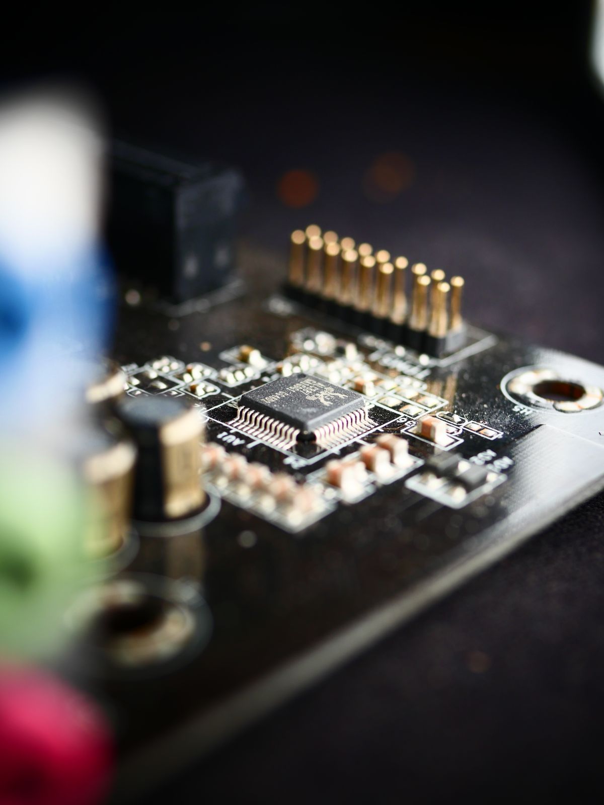
Digital return current comes next. A return path that crosses under the analogue front end couples through the plane whether or not the schematic shows a connection. Splitting the plane and placing the single tie point behind the ADC costs one review cycle and saves a respin.
Defibrillation protection then works against you. Series resistors in each input leg add their own thermal noise, which the table above already accounts for, and they add something worse: mismatch. Common-mode rejection in a real system is limited by the impedance imbalance between the two legs, not by the CMRR figure on the amplifier's front page. Two 10 kΩ protection resistors at 1% tolerance can present 200 Ω of imbalance, and mains interference converts to differential signal through that imbalance.
Mains here runs at 50 Hz. A 50 Hz notch removes the interference and takes real QRS energy with it, which distorts the morphology your classifier was trained on. Reject mains through matched impedances and a working right-leg drive, and keep the notch as the thing you never had to switch on.
Day 1 characterisation lies
Almost all published front-end characterisation happens on a signal generator through an RC phantom, at room temperature, on a board assembled that week. Every number in that setup is optimistic for a device meant to run for three weeks on a chest.
The hydrogel dries. The adhesive lifts at one corner after a shower. Sweat changes the interface chemistry and then evaporates. Movement charges the adhesive triboelectrically and dumps that charge into the input as a step the high-pass filter takes seconds to recover from. By day 18 you are running the same firmware against a different sensor.
Characterise noise on a worn electrode pulled late in the wear period, not a fresh one, and log analysable fraction by day rather than as a single figure for the whole study. If your analysable percentage does not fall across the wear period, you are not measuring it correctly.
What this costs the model
A classifier learns the noise character of whatever hardware produced the recordings it was trained on. Curated research recordings tend to come from clinical-grade equipment, prepped multi-lead placements and a technician in the room. Your patch is one lead, on a patient washing dishes, on day 16. That mismatch reaches the model as distribution shift on the input side, before a single weight is wrong.
Motion artefact is the specific danger. It is high-amplitude, irregular and broad-band, which is a description that also fits ventricular tachycardia. A model that never saw your particular motion artefact during training will not fail with low confidence. It will call VT at 0.94 and generate an alert.
That asymmetry matters more than it looks. A missed supraventricular run costs you a finding. A false VT alert costs you the cardiologist, and she only has to be wrong-footed twice before she stops trusting the automated layer and reads everything by hand, which removes the reason the device exists. Clinician trust is the scarcest resource in the whole system and false positives spend it fastest.
Every hour your device marks unanalysable is an hour of battery, adhesive, patient tolerance and clinic slot that produced nothing. Those hours cluster during movement, which is when symptomatic episodes happen. Losing 8% of a recording is not losing 8% of the diagnostic yield. It is worse, and the direction of the bias runs against you.
What to check before firmware goes near a board
Input-referred noise measured with the inputs shorted through the actual protection network, not through a short. Noise measured again with a 300 kΩ source, because that is day 14. CMRR measured with a deliberate 5% imbalance between legs, because matched electrodes are a laboratory condition. Leakage measured after 48 hours at 40 °C and 85% relative humidity on an unconformal-coated board, because that is the humidity failure and it does not appear at day zero.
None of this is exotic. It is the part of the work that decides whether the model downstream is doing classification or interpreting noise, and no amount of model capacity recovers a signal the front end never captured cleanly.